
Data Granularity:
Contents
Data Granularity:
From questions to code
While determining what measurements to make to understand a process is clearly important, the difficulty of understanding what or who to measure shouldn’t be overlooked. One needs to be clear about both the individuals being observed, along with the attributes being measured.
Example: Suppose a Data Scientist, working at video streaming platform, studies users’ viewing behavior. The data she uses might come in two possible forms:
Each row represents an event comprising of a user streaming a particular video; attributes include the user streaming the video, the name of the video, the length of the streaming event, whether the video was watched to completion, etc.
Each row represents a user; attributes include the average and total time spent streaming, how often a video was watched to completion, etc.
These datasets have different data designs; each is better suited to answer certain questions than the other. However, the user-level data is fundamentally an aggregate view of the event-level data: it gives a coarser view of the data. Below are a few differences between the two data designs.
— |
Event Level (fine) |
User Level (coarse) |
|---|---|---|
Answering questions about: |
cost of running servers |
net revenue per user |
Cost implications of data collection: |
large/expensive to store |
smaller/cheaper to store |
Privacy implications of data collection: |
possibly detailed personal data |
more easily anonymized |
Flexibility of use: |
usable for a broad range of questions |
drops more information about underlying events |
… |
… |
… |
Suppose, for example, the Data Scientist notices when looking at the user-level data that 5% of paying users accounts for 95% of all video watched on the platform. A knee-jerk response might be to discourage these users from such heavy use, as this small number of paying subscribers account for most of the costs of running the platform. However, a look at the event-level data might reveal that these users all have something in common: they watch the new live-streaming channels that the company is promoting, which consists of inordinately long events. In fact, the root of the problem lies in the service being promoted, not the users.
Data can be represented at different levels of granularity and it’s useful to move from a fine grained picture to coarser summaries while understanding what information is lost. An astute Data Scientist treats coarse grained data with skepticism, without losing the ability to effectively use it.
Group-wise operations: split-apply-combine
Moving to coarser views of a dataset involves grouping individuals into subpopulations and aggregating the measurements of the subpopulation into a table containing the aggregate summaries. This process follows the logic of split-apply-combine nicely summarized in the context of data analysis by Hadley Wickham. This data processing strategy is useful across a very broad class of computational task, allowing one to:
cleanly describe processing logic into easy-to-understand, discrete steps, and
scale a solution, using parallel processing, to large datasets.
The components of split-apply-combine are as follows:
Split the data into groups based on some criteria (often encoded in a column).
Apply function(s) to each group independently.
Combine the results into a data structure (e.g. a Series or DataFrame)
For example, given a table with group labels A, B, C in a column Col1, the sum of values in each group is calculated by splitting the table in a table for each group, summing the values in each groups’ table separately, and combining the resulting sums in a new, smaller, table (see the figure below).
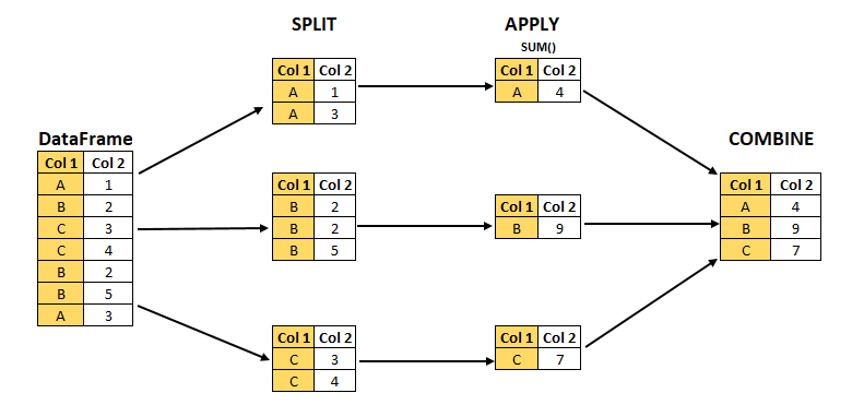
This abstraction allows one to develop transformations on a single table without worrying about the particulars of how it’s applied across groups and returned as an aggregated result.
Split: the groupby DataFrame method
In the context of Pandas DataFrames, the split-apply-combine paradigm is implemented via the DataFrameGroupBy class.
DataFrame.groupby(key) is a DataFrame method that represents the “split” portion of split-apply-combine. The DataFrameGroupBy object it returns is a dictionary like object, keyed on a (list of) column name(s) key, with values given by the indices of each group.
Example: df defined below is a DataFrame with group labels contained in Col1 and integer values in Col2 and Col3. Several useful GroupBy properties and methods are illustrated below:
df = pd.DataFrame({
    'Col1': 'A B C C B B A'.split(),
    'Col2': [1, 2, 3, 4, 2, 5, 3],
    'Col3': [4, 3, 1, 2, 4, 5, 3]
})
df
| Col1 | Col2 | Col3 | |
|---|---|---|---|
| 0 | A | 1 | 4 |
| 1 | B | 2 | 3 |
| 2 | C | 3 | 1 |
| 3 | C | 4 | 2 |
| 4 | B | 2 | 4 |
| 5 | B | 5 | 5 |
| 6 | A | 3 | 3 |
The GroupBy object does not have a descriptive string representation:
G = df.groupby('Col1')
G
<pandas.core.groupby.generic.DataFrameGroupBy object at 0x11ff2ae80>
However, the groups property returns a dictionary keyed by group label, with the indices of df corresponding to each group label:
G.groups
{'A': Int64Index([0, 6], dtype='int64'),
 'B': Int64Index([1, 4, 5], dtype='int64'),
 'C': Int64Index([2, 3], dtype='int64')}
The G.get_group(label) method returns the DataFrame df.loc[df[key] == label]:
G.get_group('A')
| Col1 | Col2 | Col3 | |
|---|---|---|---|
| 0 | A | 1 | 4 |
| 6 | A | 3 | 3 |
If the aggregation only involves one of the columns, selecting that column saves space. The resulting object is a SeriesGroupBy object, which is similar to a DataFrameGroupBy object:
G['Col2']
<pandas.core.groupby.generic.SeriesGroupBy object at 0x11a64df28>
G['Col2'].get_group('A')
0    1
6    3
Name: Col2, dtype: int64
Example: In place of a column name, groupby also accepts a function to split data into groups:
the domain of the function is the index of the DataFrame,
the groups are labeled by the image of the function,
each group consists of indices that map to the same value under the function.
For example, the following function creates a GroupBy object with three groups: Small, Medium, and Large.
def grouper(x):
    if x <= 2:
        return 'Small'
    elif 3 < x <= 4:
        return 'Medium'
    else:
        return 'Large'
(
    df
    .set_index('Col2')
    .groupby(grouper)
    .groups
)
{'Large': Int64Index([3, 5, 3], dtype='int64', name='Col2'),
 'Medium': Int64Index([4], dtype='int64', name='Col2'),
 'Small': Int64Index([1, 2, 2], dtype='int64', name='Col2')}
Apply-Combine: GroupBy methods
Recall that the ‘apply-combine’ steps consist of applying a transformation to the groups created in the ‘split’ step, followed by combining the separate results into a single data structure. Pandas GroupBy methods couple these two steps: while each method implements its own apply logic, all of them combine the transformed groups into a natural output data structure.
Many DataFrame methods also naturally extend to GroupBy objects. The Pandas documentation contains an exhaustive list.
Example: Calculating the mean of the groups of the of the simple DataFrame df defined in the previous example:
df
| Col1 | Col2 | Col3 | |
|---|---|---|---|
| 0 | A | 1 | 4 |
| 1 | B | 2 | 3 |
| 2 | C | 3 | 1 |
| 3 | C | 4 | 2 |
| 4 | B | 2 | 4 |
| 5 | B | 5 | 5 |
| 6 | A | 3 | 3 |
G = df.groupby('Col1')
G.mean()
| Col2 | Col3 | |
|---|---|---|
| Col1 | ||
| A | 2.0 | 3.5 |
| B | 3.0 | 4.0 |
| C | 3.5 | 1.5 |
Example: The table climbs contains a list of almost 4000 attempts at climbing to the summit of Mt. Rainier in Washington State, during the years 2014-2015. Each row represents a party of climbers attempting to climbing a specified route up the mountain, on a given date.
climbs
| Date | Route | Attempted | Succeeded | |
|---|---|---|---|---|
| 0 | 11/27/2015 | Disappointment Cleaver | 2 | 0 |
| 1 | 11/21/2015 | Disappointment Cleaver | 3 | 0 |
| 2 | 10/15/2015 | Disappointment Cleaver | 2 | 0 |
| ... | ... | ... | ... | ... |
| 3966 | 1/6/2014 | Disappointment Cleaver | 8 | 0 |
| 3967 | 1/5/2014 | Disappointment Cleaver | 2 | 0 |
| 3968 | 1/4/2014 | Gibraltar Ledges | 3 | 2 |
3969 rows × 4 columns
Most parties are composed of multiple climbers, as evidenced by the ‘Attempted’ column. The total number of people who attempted each route over the two year period is:
climbs.groupby('Route')['Attempted'].sum()
Route
Curtis Ridge                  4
Disappointment Cleaver    15227
Edmonds HW                    4
                          ...
Tahoma Cleaver                3
Tahoma Glacier               33
Wilson Headwall               5
Name: Attempted, Length: 23, dtype: int64
Notice the resulting Series is sorted by the grouping key; there are 24 routes sorted alphabetically.
To calculate the routes with the most climbers on a given day, group the climbs by both date and route name:
(
    climbs
    .groupby(['Date', 'Route'])['Attempted']
    .sum()
    .sort_values(ascending=False)
    .reset_index()
)
| Date | Route | Attempted | |
|---|---|---|---|
| 0 | 7/25/2014 | Disappointment Cleaver | 182 |
| 1 | 6/26/2015 | Disappointment Cleaver | 144 |
| 2 | 7/3/2015 | Disappointment Cleaver | 135 |
| ... | ... | ... | ... |
| 943 | 5/28/2015 | Kautz Glacier | 1 |
| 944 | 6/13/2015 | Kautz Glacier | 1 |
| 945 | 8/8/2015 | Emmons-Winthrop | 1 |
946 rows × 3 columns
Remark: Grouping on multiple columns results in a multi-indexed Series/DataFrame; using reset_index on the output simplifies further processing.
Similarly to the case of DataFrames, the GroupBy method agg applies columnar Series methods to the groups of a GroupBy object. Compare how each of the following outputs relates to the analogous DataFrame method.
Passing a list of functions applies each function to each column of each group
Passing a dictionary of functions applies the functions to the specified column in each group.
Example: Using agg quickly creates a compact table of descriptive statistics of the attempts up the routes on Mt. Rainier:
climbs.groupby('Route').agg(['count', 'sum', 'mean', np.median, 'max'])
| Attempted | Succeeded | |||||||||
|---|---|---|---|---|---|---|---|---|---|---|
| count | sum | mean | median | max | count | sum | mean | median | max | |
| Route | ||||||||||
| Curtis Ridge | 2 | 4 | 2.000000 | 2.0 | 2 | 2 | 2 | 1.000000 | 1.0 | 2 |
| Disappointment Cleaver | 2720 | 15227 | 5.598162 | 4.0 | 12 | 2720 | 8246 | 3.031618 | 2.0 | 12 |
| Edmonds HW | 2 | 4 | 2.000000 | 2.0 | 2 | 2 | 0 | 0.000000 | 0.0 | 0 |
| ... | ... | ... | ... | ... | ... | ... | ... | ... | ... | ... |
| Tahoma Cleaver | 1 | 3 | 3.000000 | 3.0 | 3 | 1 | 3 | 3.000000 | 3.0 | 3 |
| Tahoma Glacier | 11 | 33 | 3.000000 | 3.0 | 5 | 11 | 11 | 1.000000 | 0.0 | 3 |
| Wilson Headwall | 2 | 5 | 2.500000 | 2.5 | 3 | 2 | 0 | 0.000000 | 0.0 | 0 |
23 rows × 10 columns
The columns of the output are multi-indexed, as each function is applied to both the ‘Attempted’ and ‘Succeeded’ columns of the DataFrames of each route. For example, the DataFrame lists ‘Disappointment Cleaver’ was:
attempted by 2720 climbing parties,
attempted by a total of 15227 climbers,
a total of 8246 climbers successfully made it to the summit by the route,
the average party size attempting the route was 5.59 climbers.
Notice that the Date column was dropped from the output; Pandas drops non-numeric columns when any of the aggregation methods requires numeric data. Passing a dictionary of aggregations into agg allows for a more tailored set of aggregations:
climbs.groupby('Route').agg({'Attempted':['mean', 'max'], 'Date': ['max']})
| Attempted | Date | ||
|---|---|---|---|
| mean | max | max | |
| Route | |||
| Curtis Ridge | 2.000000 | 2 | 6/12/2015 |
| Disappointment Cleaver | 5.598162 | 12 | 9/9/2015 |
| Edmonds HW | 2.000000 | 2 | 9/14/2014 |
| ... | ... | ... | ... |
| Tahoma Cleaver | 3.000000 | 3 | 6/5/2015 |
| Tahoma Glacier | 3.000000 | 5 | 8/2/2014 |
| Wilson Headwall | 2.500000 | 3 | 4/26/2015 |
23 rows × 3 columns
Generic Apply-Combine: apply method
The apply method is the most general GroupBy method; it applies any function defined on the ‘grouped’ dataframes and attempts to combined the result into meaningful output. While very flexible, the apply method is slower, less space efficient, and more prone to error than using standard GroupBy methods; it should be avoided when possible.
Use this method when either:
the transformation depends on complicated group-wise conditions on multiple columns.
the output dimensions of the resulting Series/DataFrame are nonstandard.
Example: For the dataframe df, generate a dataframe indexed by label Col1, with five of random integers chosen within the range of values of Col2 within the group. For example, within the A group Col2 contains 1, 3; the output row with index A should therefore contain five randomly chosen integers between 1 and 3.
df
| Col1 | Col2 | Col3 | |
|---|---|---|---|
| 0 | A | 1 | 4 |
| 1 | B | 2 | 3 |
| 2 | C | 3 | 1 |
| 3 | C | 4 | 2 |
| 4 | B | 2 | 4 |
| 5 | B | 5 | 5 |
| 6 | A | 3 | 3 |
Define a function that takes in a group-dataframe (i.e. retrievable by df.groupby('Col1').get_group(label)), calculates the minimum and maximum values of Col2 within that group, and returns the random integers as a Series:
def generate_random(gp):
    n_rand = 5
    m, M = gp['Col2'].min(), gp['Col2'].max()
    r = np.random.randint(m, M, size=n_rand)
    return pd.Series(r, index=['rand_%d' % (x + 1) for x in range(n_rand)])
The apply method combines these Series of random integers into a DataFrame indexed by label:
G.apply(generate_random)
| rand_1 | rand_2 | rand_3 | rand_4 | rand_5 | |
|---|---|---|---|---|---|
| Col1 | |||||
| A | 1 | 2 | 2 | 1 | 1 |
| B | 2 | 4 | 2 | 2 | 4 |
| C | 3 | 3 | 3 | 3 | 3 |
Another common use case for apply is when the output DataFrame has the same index as the input DataFrame. This often occurs when the elements of a table need to be scaled by a groupwise condition.
Example (transform): Scale the DataFrame linearly, so that an entry is represented as the proportion of the range for each group. For example, in ‘Col3’, the ‘B’ group has values 3, 4, 5. The range of the ‘B’ group is (5 - 3) = 2. The value 4 is halfway is in the middle of the range and thus is scaled to 0.5.
df
| Col1 | Col2 | Col3 | |
|---|---|---|---|
| 0 | A | 1 | 4 |
| 1 | B | 2 | 3 |
| 2 | C | 3 | 1 |
| 3 | C | 4 | 2 |
| 4 | B | 2 | 4 |
| 5 | B | 5 | 5 |
| 6 | A | 3 | 3 |
def scale_by_range(gp):
    rng = gp.max() - gp.min()
    from_min = gp - gp.min()
    return from_min / rng
The function scale_by_range returns a DataFrames of the same index as the input. Pandas thus aligns them by common columns, returning a dataframe of the same shape as df:
G.apply(scale_by_range)
| Col2 | Col3 | |
|---|---|---|
| 0 | 0.0 | 1.0 |
| 1 | 0.0 | 0.0 |
| 2 | 0.0 | 0.0 |
| 3 | 1.0 | 1.0 |
| 4 | 0.0 | 0.5 |
| 5 | 1.0 | 1.0 |
| 6 | 1.0 | 0.0 |
Pandas provides a method specifically for this pattern: transform. It’s appropriate when passing a function to apply that returns a Series/DataFrame with the same index as the input. This method is both faster and less error prone than using apply in this case.
G.transform(scale_by_range)
| Col2 | Col3 | |
|---|---|---|
| 0 | 0.0 | 1.0 |
| 1 | 0.0 | 0.0 |
| 2 | 0.0 | 0.0 |
| 3 | 1.0 | 1.0 |
| 4 | 0.0 | 0.5 |
| 5 | 1.0 | 1.0 |
| 6 | 1.0 | 0.0 |
Example: Among the 24 routes up Mt. Rainier, only a few of them see more than 15 attempts in 2014-15. The apply method can be used to filter out all attempts on routes that aren’t very popular (fewer than 15 attempts in 2014-15). The split-apply-combine logic:
splits the table into separate routes on the mountain (split),
checks the size of each table (apply):
leaving the table untouched if it contains at least 15 rows,
otherwise, omitting the rows (returning an empty DataFrame)
Aggregating the (possibly empty) DataFrames into a filtered subtable of the original
climbs.
def filter_few(df, min_size=15):
    '''return df if it has at least `min_size` rows,
    otherwise return an empty dataframe with the same columns'''

    if df.shape[0] >= min_size:
        return df
    else:
        return pd.DataFrame(columns=df.columns)
popular_climbs = (
    climbs
    .groupby('Route')
    .apply(filter_few)
    .reset_index(level=0, drop=True) # drop group key: Route
)

popular_climbs.sort_index()
| Date | Route | Attempted | Succeeded | |
|---|---|---|---|---|
| 0 | 11/27/2015 | Disappointment Cleaver | 2 | 0 |
| 1 | 11/21/2015 | Disappointment Cleaver | 3 | 0 |
| 2 | 10/15/2015 | Disappointment Cleaver | 2 | 0 |
| ... | ... | ... | ... | ... |
| 3966 | 1/6/2014 | Disappointment Cleaver | 8 | 0 |
| 3967 | 1/5/2014 | Disappointment Cleaver | 2 | 0 |
| 3968 | 1/4/2014 | Gibraltar Ledges | 3 | 2 |
3914 rows × 4 columns
The resulting table is a filtered subtable of the original table. To verify all routes contained in popular_climbs have at least 15 attempts, we can calculate the distribution of routes:
popular_climbs['Route'].value_counts()
Disappointment Cleaver    2720
Emmons-Winthrop            631
Kautz Glacier              181
                          ...
Liberty Ridge               69
Ingraham Direct             53
Ptarmigan Ridge             22
Name: Route, Length: 9, dtype: int64
Example: This pattern is common enough that Pandas provides the filter method to optimize this computation. The filter method takes in a boolean ‘filtering function’ as input. The filter method keeps a grouped DataFrame exactly when the filter function returns True. Repeating the prior example, to filter out all but the popular climbing routes:
climbs.groupby('Route').filter(lambda df:df.shape[0] >= 15)
| Date | Route | Attempted | Succeeded | |
|---|---|---|---|---|
| 0 | 11/27/2015 | Disappointment Cleaver | 2 | 0 |
| 1 | 11/21/2015 | Disappointment Cleaver | 3 | 0 |
| 2 | 10/15/2015 | Disappointment Cleaver | 2 | 0 |
| ... | ... | ... | ... | ... |
| 3966 | 1/6/2014 | Disappointment Cleaver | 8 | 0 |
| 3967 | 1/5/2014 | Disappointment Cleaver | 2 | 0 |
| 3968 | 1/4/2014 | Gibraltar Ledges | 3 | 2 |
3914 rows × 4 columns
Remark: The same filtering is possible by a two step process that avoids a groupby, via:
use the empirical distribution of routes to create an array of ‘popular routes’
filter the original
climbsDataFrame using a boolean array created with theisinDataFrame method.
Try this! Of course, calculating an empirical categorical distribution on a Series, using value_counts(), is logically equivalent to splitting by Route and taking the size of each group; this approach is more memory efficient, though slower.