Combining Data: Attributes¶

Combining different measurements over the same individuals¶

Adding additional attributes to an existing dataset is often necessary to improve the description of the data generating process and answer the questions being asked of the data. In its most simple form, such a task consists of tables of the same individuals, with different attributes, collected for different purposes.

Such a process simply needs to add the columns of the second table to the first table. However, this process only works when the rows of the two tables correspond to the same individuals. Assuming a one-to-one correspondence between the individuals in the two tables, identified by their index, combining the columns of the two tables requires two steps:

sorting each table by their respective indexes (i.e. lining them up),
iterating through the (common) index of each table, combining the attributes of each row into a new table.

Remark 1: This procedure is implicitly done by Pandas whenever setting a Series as a new column of an existing DataFrame.

Remark 2: Understanding the internals of this procedure is important for both being able to debug performance issues, as well as implement custom procedures when the correspondence between the rows of the tables is not obvious.

This procedure is known as joining or merging tables (column-wise). The correspondence between the rows (e.g. via a shared index) is called a join key.

Example: Below, two tables contain characteristics of California counties obtained from the US Census: one contains a population attribute, the other contains the median household income. The join key is the ‘County’ column.

Joining data column-wise¶

Pandas has multiple ways of executing a (column-wise) join of DataFrames. Below outlines each and their relative advantages. In spite of the options, one should use the merge method whenever possible!

Join Technique 1: column(s) assignment The most simple way of joining the columns of two tables along a shared index is by column(s) assignment. If df1 and df2 have indexes in one-to-one correspondence, they can be joined via:

df1[df2.columns] = df2

This technique is simple and space efficient, since column assignment modifies the left-hand DataFrame in-place. However it has many disadvantages:

Advantages	Disadvantages
Space Efficient	Doesn’t work with the method chaining
—	Joining more than two DataFrames requires multiple lines
—	Works only when indexes are in one-to-one correspondence
—	Sorts the two DataFrames by index, even if already aligned

Join Technique 2 (concat): The Pandas function concat column-wise joins a list of DataFrames by a shared index, with several convenient keyword arguments. If df1,...,dfN are DataFrames, then the columns of these DataFrames can be joined by passing them to concat in a list:

pd.concat([df1, ..., dfN], axis=1)

This function has many advantages over column assignment:

Advantages	Disadvantages
Can easily join many DataFrames	Doesn’t work with method chaining
Indexes don’t need to be 1-1 correspondence	The DataFrames must of a common index
Can skip sorting indexes by setting `ignore_index=True`

Join Technique 3 (merge): The merge method is the most flexible joining technique in Pandas. By default, it joins the columns of two DataFrames on common columns. If df1,...,dfN are DataFrames with shared columns that identify observations between them, the DataFrames can be joined by chaining together successive merge calls:

df1.merge(df2).merge(df3)...merge(dfN)

If the DataFrames have a shared index, then merge is called with the left_index/right_index=True keyword argument.

Advantages	Disadvantages
Works with method chaining	Can’t pass an arbitrary list of DataFrames
Join key doesn’t need to be in index	Can’t skip sorting by the join key
Rows don’t need to be 1-1 correspondence

Example:

counties = pop_counties.merge(inc_counties)
counties

	County	Population	Income
0	Calaveras	44921	54936
1	San Diego	3183143	63996
2	San Joaquin	701050	53253
...	...	...	...
55	Marin	256802	91529
56	Monterey	424927	58582
57	San Mateo	739837	91421

58 rows × 3 columns

Check the relative sizes of the inputs confirm every row has its expected match. The input tables exactly one entry for each of the 58 California counties; the joined table should have one row per county and three columns.

print(pop_counties.shape, inc_counties.shape, counties.shape, sep='\n')

(58, 2)
(58, 2)
(58, 3)

Remark: this simple check can save hours of debugging!

Join types¶

Not uncommonly, when joining two tables, the observations don’t perfectly align. In these cases, care must be taken with the approach to joining the observations. There are three possibilities:

the observations are in one-to-one correspondence,
one of the tables contains observations not contained in the other,
both of the tables contain observations missing in the other.

In the first case, there is no ambiguity in combining the two tables. However, in the latter two cases, one has to decide whether to retain the observations that are present in only one of the tables. These cases are enumerated in the following join types.

Given two tables, the possible join types of a combined table are:

An inner join keeps only the observations with a matched join key,
An outer join keeps all observations, even if not-matched,
A left join keeps all observations in the left table,
A right join keeps all observations in the right table.

Below, the join types are illustrated with Venn diagrams; the diagrams overlap if the tables share an observation:

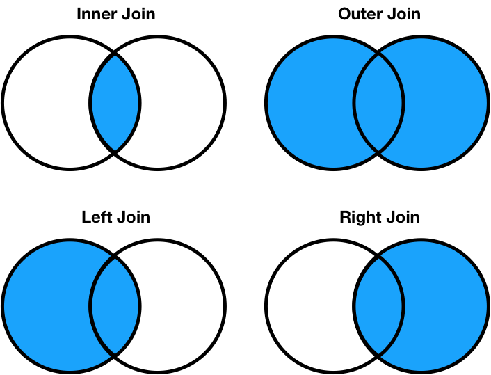
The default operation is typical as inner join, as is true for the merge method.

Example: Suppose the county population table only includes information on counties with populations over 1.5M residents. The inner-join between this partial population table and the full income table will drop income information!

The partial population file only contains seven of the 58 counties:

partial_pop = pop_counties.loc[pop_counties['Population'] > 1.5*10**6]
partial_pop

	County	Population
1	San Diego	3183143
9	Riverside	2266899
18	Santa Clara	1841569
24	San Bernardino	2078586
37	Los Angeles	9974203
50	Alameda	1559308
53	Orange	3086331

The inner-join only contains the seven large population counties, even though the income table contains all 58 counties:

partial_pop.merge(inc_counties)

	County	Population	Income
0	San Diego	3183143	63996
1	Riverside	2266899	56592
2	Santa Clara	1841569	93854
3	San Bernardino	2078586	54100
4	Los Angeles	9974203	55870
5	Alameda	1559308	73775
6	Orange	3086331	75998

A right-join retains all the income values and adds population entries when available; a NaN value appears when a corresponding county doesn’t appear in the population table:

partial_pop.merge(inc_counties, how='right')

	County	Population	Income
0	San Diego	3183143.0	63996
1	Riverside	2266899.0	56592
2	Santa Clara	1841569.0	93854
...	...	...	...
55	San Benito	NaN	67874
56	Yolo	NaN	55508
57	Lassen	NaN	53351

58 rows × 3 columns

Example: Joins in Pandas are exact matches between join keys, including a match on the data type. For example, columns with integer columns, with one of them typed as a string, will fail to properly join. These mistakes are hard to spot, as Pandas hides the type of the contents of DataFrames on formating.

Defining two dataframes with matching indexes of different types:

df_ints = pd.DataFrame({'B': range(0, 6, 2)}, index=[0, 1, 2])
df_strs = pd.DataFrame({'C': range(0, 12, 4)}, index='0 1 2'.split())

Joining the two DataFrames with an outer-join illustrates the failure to join on index:

merged = df_ints.merge(df_strs, right_index=True, left_index=True, how='outer')
merged

	B	C
0	0.0	NaN
1	2.0	NaN
2	4.0	NaN
0	NaN	0.0
1	NaN	4.0
2	NaN	8.0

The index of the merged table contains distinct values of both integer and string type:

merged.index

Index([0, 1, 2, '0', '1', '2'], dtype='object')

Example: By default, merge sets the join-key to the set of all common columns between the DataFrames being merged, sometimes leading to unintended consequences when both tables share similar attributes. The join-key can be specified explicitly using the keyword on.

The DataFrames df1 and df2 have different resulting joins when the join key is column ‘A’ vs. columns (‘A’, ‘B’):

df1 = pd.DataFrame({'A': range(3), 'B': range(0, 6, 2)})
df2 = pd.DataFrame({'A': range(3), 'B': range(0, 12, 4)})

df1.merge(df2)

	A	B
0	0	0

df1.merge(df2, on='A', suffixes=['_1','_2'])

	A	B_1	B_2
0	0	0	0
1	1	2	4
2	2	4	8

Remark: The suffixes argument decorates the duplicate column names with which table the column originated from.

Example: When joining new attributes to a dataset under investigation, the additional information isn’t always available for the complete population. For example, when investigating the incomes by California county, suppose one attempts to join demographic information (such as population size) to the incomes dataset. However, if this demographic information is only available for counties with a large population, the merge dataset will exhibit significant bias:

large_pop = pop_counties.loc[pop_counties['Population'] > 200000]

Upon merging the incomes with the demographics, an inner-join drops all counties of small size. The resulting average income is quite different than the average income across all counties:

inc_counties.merge(large_pop)['Income'].mean()

63668.57142857143

inc_counties['Income'].mean()

56034.362068965514

By using an left-join, on can avoid dropping these observations (at the expense of introducing missing values into the merged dataset):

inc_counties.merge(large_pop, how='left')['Income'].mean()

56034.362068965514

Many-to-one joins¶

A join performed on a join-key with duplicate entries results in either a ‘many-to-one’ or a ‘many-to-many’ join. Though these joins occur naturally, the resulting datasets might initially seem unintuitive.

Many-to-one joins occur naturally when using ‘lookup tables’ to attach richer information about an attribute of a dataset (as opposed to an individual). For example, a table might include the purchase history of customers subscribing to a music-streaming service:

Customer	Plan Type
23523	Premium
43453	Premium
34523	Student
…	…
98345	Family
13423	Premium
34234	Student

Computing the total revenue generated from these purchases, one needs to merge this table with the three-row table of plan types:

Plan Type	Price
Student	$4.99
Premium	$9.99
Family	$14.99

A few observations on how this join differs from the simple joins covered before:

the join-key ‘Plan Type’ is an attribute of the table, not an identifier for the observations of the tables.
one expects the resulting joined table to contain the price next to each customer purchase; the each row in the small table is repeated many times over.

The result of joining these two tables is:

Customer	Plan Type	Price
23523	Premium	$9.99
43453	Premium	$9.99
34523	Student	$4.99
…	…	…
98345	Family	$14.99
13423	Premium	$9.99
34234	Student	$4.99

Example: The dataset cities contains population and income information on 1442 California cities, along with the name of the county to which each city belongs. Using this dataset, one can roughly calculate which cities make significantly more or less than their neighbors: create a derived attribute using the ratio of the average household income of a given city to the average household income of the county in which it lies.

cities

	City	County	Population	Income
0	Acalanes Ridge	Contra Costa	1226	160000.0
1	Acampo	San Joaquin	776	141250.0
2	Acton	Los Angeles	6956	92245.0
...	...	...	...	...
1439	Yucaipa	San Bernardino	52406	58506.0
1440	Yucca Valley	San Bernardino	21083	43086.0
1441	Zayante	Santa Cruz	853	81308.0

1442 rows × 4 columns

Calculating this attribute requires joining the county dataset with the city dataset on the ‘County’ attribute. Since possibly many cities belong to the same county, this is a many-to-one join.

cities_with_county_info = cities.merge(counties, on='County', suffixes=['_city', '_county'])
cities_with_county_info

	City	County	Population_city	Income_city	Population_county	Income_county
0	Acalanes Ridge	Contra Costa	1226	160000.0	1081232	79799
1	Alamo	Contra Costa	15639	163151.0	1081232	79799
2	Alhambra Valley	Contra Costa	499	62000.0	1081232	79799
...	...	...	...	...	...	...
1435	San Juan Bautista	San Benito	2219	57717.0	56888	67874
1436	Tres Pinos	San Benito	457	75893.0	56888	67874
1437	San Francisco	San Francisco	829072	78378.0	829072	78378

1438 rows × 6 columns

Remark: What happens if the join key were not specified in the merge? What condition must be met for a city to belong to the merged table?

Once merged, the ‘income ratio’ attribute is simply the ratio of two columns. The cities with the highest income ratios are small gated communities within Los Angeles County:

(
    cities_with_county_info.assign(
        income_ratio=cities_with_county_info['Income_city'] / cities_with_county_info['Income_county']
    ).sort_values(by='income_ratio', ascending=False)
)

	City	County	Population_city	Income_city	Population_county	Income_county	income_ratio
134	Hidden Hills	Los Angeles	1749	245694.0	9974203	55870	4.397602
177	Rolling Hills	Los Angeles	1689	218583.0	9974203	55870	3.912350
169	Palos Verdes Estates	Los Angeles	13568	171328.0	9974203	55870	3.066547
...	...	...	...	...	...	...	...
595	Boulevard	San Diego	434	12421.0	3183143	63996	0.194090
1301	Valley Ford	Sonoma	167	9312.0	491790	63799	0.145958
526	Verdi	Sierra	92	4853.0	3019	43107	0.112580

1438 rows × 7 columns

Many-to-many joins¶

Recall that, assuming a one-to-one correspondence between the individuals in the two tables, joining the columns of the two tables requires two steps:

sorting each table by their respective join-keys (i.e. lining them up),
iterating through the (common, corresponding) rows of each table, combining the attributes of each row into a new table.

Now, consider if one, or both, of the tables contains duplicate values in the column specified as the join-key. How does step 2 change? Sketch out an algorithm. How many rows does the resulting joined table have?

Broadcast join¶

When one of the tables being joined is small, it’s faster to use a broadcast join. Broadcast joins use the following procedure:

load the small table into a dictionary $D$, keyed by the join-key.
iterate through the large table; for each row $r$ in the table:
1. access the join key $k$ for that row,
2. get the value $v = D[k]$ corresponding to this key,
3. append the value $v$ from the dictionary to the row $r$.

This procedure is fast:

it doesn’t require sorting either table,
dictionary lookups only require constant time,

So this sorting algorithm runs in a time proportional to the sum of the lengths of the two tables.

Example: Given the two tables of streaming music purchases (purchases), and the prices of each plan type (prices), one can use a broadcast join to combine the two tables on ‘Plan Type’:

D = prices.set_index('Plan Type').to_dict()
purchases['Price'] = purchases.apply(lambda x:D.get(x['Plan Type']))

Data Science in Practice

Combining Data: Attributes

Contents